Checking solutions with this helpful discussion and this other set of solutions. Yay for open learning.
# pandan::pandan_view(project = "rethinking", distill = TRUE, update = FALSE)easy
2E1
Which of the expressions below correspond to the statement: the probability of rain on Monday?
- P(rain)
- P(rain|Monday)
- P(Monday|rain)
- P(rain, Monday) / P(Monday)
Adapting the equation on p. 37 to a more generalised statement, for a parameter of interest \(\theta\) and observations \(y\) dependent on that parameter, we have
\[ P(\theta | y) = \frac{P(y|\theta)P(\theta)}{P(y)} = P(\theta, y)/P(y) \]
Then P(rain|Monday) = P(rain, Monday) / P(Monday).
So, I conclude that 2. and 4. correspond to the statement.
2E2
The following statement corresponds to the expression P(Monday|rain):
- The probability that it is Monday, given that it is raining.
2E3
The probability that it is Monday given that it is raining.
Can be expressed
P(Monday|rain) = P(rain|Monday)P(Monday)/P(rain)
So, the following statements correspond.
- P(Monday|rain) and 4. P(rain|Monday)P(Monday)/P(rain)
2E4
The Bayesian statistician Finetti began his book on probablity theory with the declaration: “PROBABILITY DOES NOT EXIST”. What he meant is that probability is a device for describing uncertainty from the perspective ofg an observer with limited knowledge; it has no objective reality. What does it mean to say, “the probability of water is 0.7”?
Based on the observations we have of water and land from globe tossing, the most credible proportion of the globe is approximately 0.7.
medium
2M1
Compute and plot the grid approximate posterior distribution for each of the following sets of observations. In each case, assume a uniform prior for p.
- WWW
- WWWL
- LWWLWWW
We assume \[ \begin{array} \\W & \sim & \text{binomial}(N, p)\\ p & \sim & \text{uniform}(0, 1) \end{array} \] where \(W\) is the number of water observations and \(N = L + W\) is the total number of water and land observations. We only know \(p\) is a proportion, so we know that it falls in \([0,1]\).
We are interested in finding \[ P(p|W,L) = P(W,L|p)P(p)/P(W,L) \] where \(P(p|W,L)\) is the posterior, \(P(W,L|p)\) is the probability of the data, \(P(W,L)\) is the prior.
\[ \text{Posterior} = \frac{ \text{Probability of the data} \times \text{Prior} }{ \text{Average probability of the data} } \]And this is Bayes’ theorem. It says the the probability of any particular value of \(p\), considering the data is equal to the product of the relative plausibility of the data, conditional on \(p\), and the prior plausibility of \(p\), divided by the average probability of the data.
library(tidyverse)

# set number of points for the grid
n <- 10

# create a grid approximation tableT
www <-
    tibble(
        # define grid
        p = seq(0, 1, length.out = n),
        # compute prior at each parameter value
        prior = 1
    ) %>%
    mutate(
        # compute the likelihood at each parameter value
        plausibility = dbinom(3, size = 3, prob = p),
        # comput the unstandardised posterior
        unstd_post = plausibility * prior,
        # standardise the posterior
        posterior = unstd_post / sum(unstd_post)
    )
grid_plot <- function(post_df, title_text) {
post_df %>%
ggplot(
aes(
x = p,
y = posterior
)
) +
geom_line(alpha = 0.4) +
geom_point(alpha = 0.8) +
labs(title = title_text) +
ggthemes::theme_tufte()
}It makes sense that for www observation, we have a
monotonically increasing posterior. Higher values of \(p\) are more likely, given we have
only observed water.
grid_plot(www, "w w w")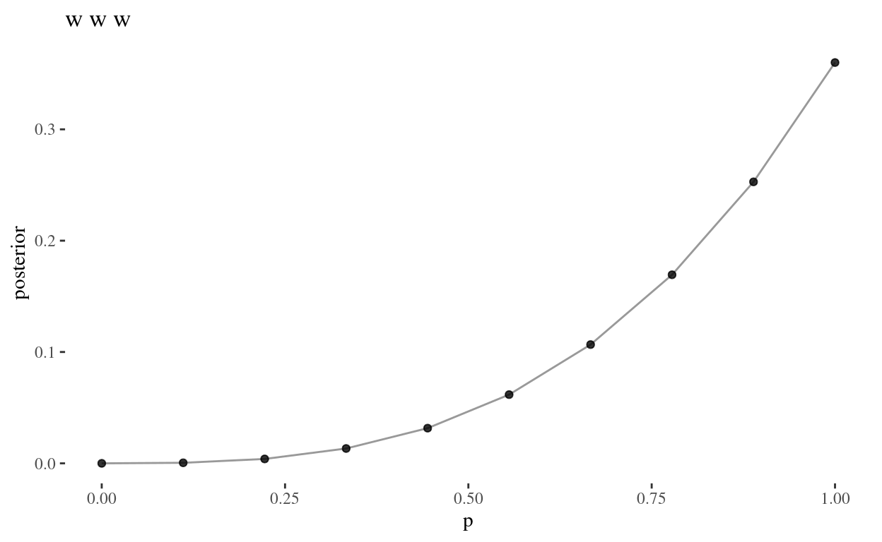
Now for the second set of observations, wwwl. This
should be slightly more interesting, as there is one land observation,
so we know with certainty that \(p \neq
1\), whereas in www, this was the most plausible
value for \(p\).
wwwl <-
    tibble(
        # define grid
        p = seq(0, 1, length.out = n),
        # compute prior at each parameter value
        prior = 1
    ) %>%
    mutate(
        # compute the likelihood at each parameter value
        plausibility = dbinom(3, size = 4, prob = p),
        # comput the unstandardised posterior
        unstd_post = plausibility * prior,
        # standardise the posterior
        posterior = unstd_post / sum(unstd_post)
    )

grid_plot(wwwl, "w w w l")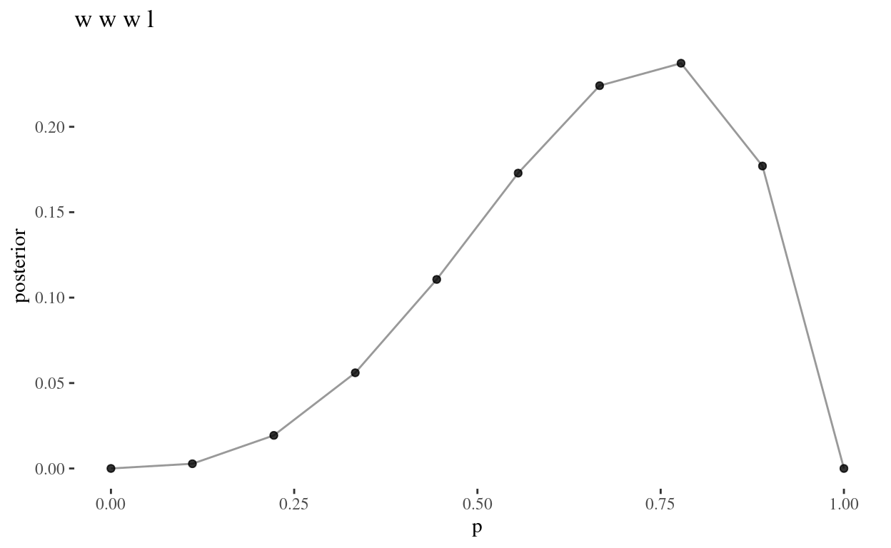
lwwlwww <-
    tibble(
        # define grid
        p = seq(0, 1, length.out = n),
        # compute prior at each parameter value
        prior = 1
    ) %>%
    mutate(
        # compute the likelihood at each parameter value
        plausibility = dbinom(5, size = 7, prob = p),
        # comput the unstandardised posterior
        unstd_post = plausibility * prior,
        # standardise the posterior
        posterior = unstd_post / sum(unstd_post)
    )

grid_plot(lwwlwww, "l w w l w w")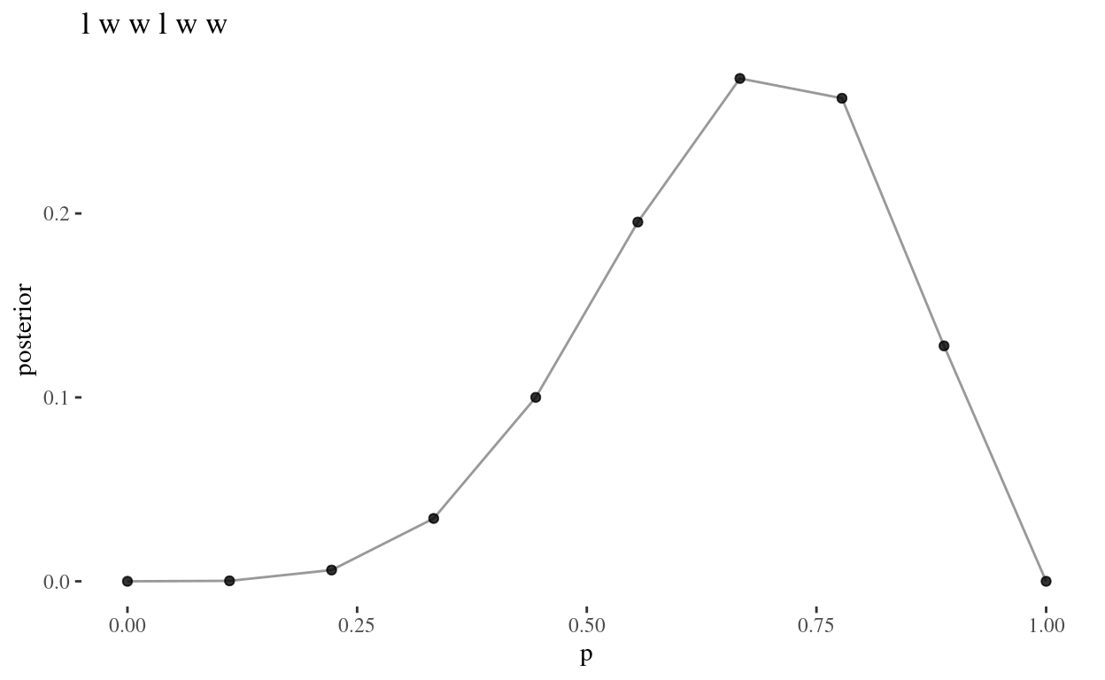
2M2
We now assume a prior \(P: [0,1] \to \{0, \theta\}\) such that \[ p \mapsto \begin{cases} 0 & p < 0.5\\ \theta & p \geqslant 0.5 \end{cases} \] where \(\theta \in \mathbb R^+\), and again compute the grid approximations as in 2M1.
Now I’ve got the general idea of each line of the grid approximation, I’ll now functionalise it.
grid_theta <- function(w, sample_size) {
  # get a random positive value
  theta <- runif(1, 1, 10000)

  # return tibble of grid approx
     tibble(
        # define grid
        p = seq(0, 1, length.out = n),
        # compute prior at each parameter value
        prior = if_else(p < 0.5, 0, theta)
    ) %>%
    mutate(
        # compute the likelihood at each parameter value
        plausibility = dbinom(w, size = sample_size, prob = p),
        # comput the unstandardised posterior
        unstd_post = plausibility * prior,
        # standardise the posterior
        posterior = unstd_post / sum(unstd_post)
    )
}
# www
grid_theta(3, 3) %>%
grid_plot("w w w, prior = 0 for p < 0.5")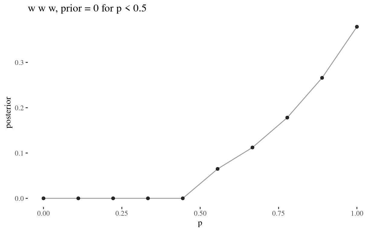
# wwwl

grid_theta(3, 4) %>%
  grid_plot("w w w l, prior = 0 for p < 0.5")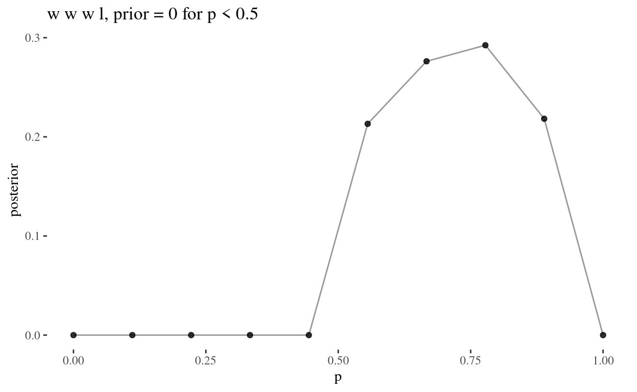
# lwwlwww
grid_theta(5, 7) %>%
  grid_plot("l w w l w w w, prior = 0 for p < 0.5")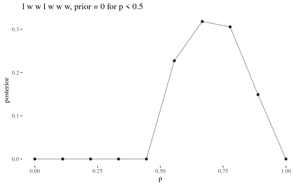
Since \[ \text{Posterior} = \frac{ \text{Probability of the data} \times \text{Prior} }{ \text{Average probability of the data} } \] In all three questions, for \(p< 0.5\), the posterior is 0.
Since the numerator is a product of the probability of the data and the prior, which is set to 0 for \(p < 0.5\), and any product containing zero is zero, we have a posterior of 0 for all values \(p < 0.5\). That is, where the prior is 0, this will always produce a posterior of 0, regardless of the value of the probability of the data.
2M3
Suppose there are two globes, one for Earth and one for Mars. The Earth globe is 70% covered in water. The Mars globe is 100% land.
So, P(water|Earth) = 0.7 and P(land|Mars) = 1.0.
Further suppose that one of these globes - you don’t know which - was tossed in the air and produced a land observation. Assume each globe was equally likely to be tossed.
So, P(Earth) = 0.5 and P(Mars) = 0.5.
Show that the posterior probability that the globe was Earth conditional on seeing land is 0.23, that is, P(Earth|land) = 0.23.
We wish to show that P(Earth|land) = 0.23.
Well, Bayes’ theorem gives us,
P(Earth|land) = P(land|Earth)P(Earth)/P(land).
So we need to find P(land|Earth), P(Earth), and P(land).
We know P(Earth) = 0.5.
Now P(water|Earth) = 0.7, so P(land|Earth) = 0.3, since there are only two possibilities on Earth.
Finally, for P(land), we note that, going back to the original generalised notation, \[ P(y) = E(P(y|\theta)) = \int P(y|\theta)P(\theta)d\theta \] so, since in this example we are dealing with discrete possibilities,
P(land) = E(P(land|Planet)) = \(\displaystyle\sum_{\text{Planet } \in \{\text{Earth},\text{Mars}\}}\) P(land|Planet)P(planet) = P(land|Earth) P(Earth) + P(land|Mars) P(Mars).
Then P(land) is
0.3 * 0.5 + 1 * 0.5[1] 0.65So, we have P(land|Earth), by Bayes’ theorem, is
(0.3 * 0.5)/(0.3 * 0.5 + 1 * 0.5)[1] 0.23076922M4
Suppose you have a deck with only three cards.
Let \(X\) denote the set of three cards, so \(|X|=3\).
And each side is either black or white. One card has two black sides. The second card has one black and one white side. The third card has two white sides.
So, we could say \(X = \{BB, BW, WW\}\).
Someone pulls out a card and places it flat on a table. A black side is shown facing up, but you don’t know the colour of the side facing down.
Let \(y\) denote the observation \(B\). Now, clearly \(P(B|WW) = 0\).
Use the counting method from Section 2. This means counting up the ways that each card could produce the observed data.
Show that the probability that the other side is also black is 2/3.
We wish to show that \(P(BB|B) = 2/3\).
tibble(
  # possible cards
  conjecture = c("BB", "BW", "WW"),
  # probability of each card
  p = rep(1 / 3, 3),
  # ways the card can produce the observation B
  ways = c(2, 1, 0)
) %>%
  # calculate the plausibility
  mutate(prod = p * ways,
         plausibility = prod / sum(prod)) %>%
  gt() %>%
  cols_label(
    conjecture = "possible cards",
    p = "likelihood of drawing card",
    ways = "ways card can produce B",
    prod = "p x ways",
    plausibility = "plausbility - p x ways/sum(p x ways)"
  ) %>%
  data_color(
    columns = vars(plausibility),
    colors = scales::col_bin(
      palette = c("#93a1a1", "white"),
      bins = 2,
      domain = NULL,
      reverse = TRUE
    )
  ) %>%
  data_color(
    columns = vars(conjecture),
    colors = scales::col_factor(
      palette = c("#93a1a1", "white", "white"),
      domain = NULL
    )
)| possible cards | likelihood of drawing card | ways card can produce B | p x ways | plausbility - p x ways/sum(p x ways) |
|---|---|---|---|---|
| BB | 0.3333333 | 2 | 0.6666667 | 0.6666667 |
| BW | 0.3333333 | 1 | 0.3333333 | 0.3333333 |
| WW | 0.3333333 | 0 | 0.0000000 | 0.0000000 |
2M5
Now suppose there are four cards \(\{BB, BW, WW, BB\}\).
Again calculate the probability the other side is black.
This time I’ll use TeX so I can see how I worked it on paper.
\[ \begin{array}{cccc} \text{possible card} & \text{chance of card} & \text{ways card produces B} & \text{chance} \times \text{ways} & \text{plausibility (product / $\Sigma$)}\\ \hline BB & 1/2 & 2 & 1 & 4/5\\ BW & 1/4 & 1 & 1/4 & 1/5\\ WW & 1/4 & 0 & 0 & 0\\ \hline &&&\Sigma = 5/4 \end{array} \]
So, the probability the other side is black is
4/5[1] 0.82M6
Imagine the black ink is heavy, and so cards with black sides are heavier than cards with white sides.
So, P(B) < P(W).
Again assume there are three cards \(\{BB, BW, WW\}\). After experimenting a number of times, you conclude that for every way to pull the \(BB\) card from the bag, there are 2 ways to pull the BW card, and 3 ways to pull the WW card. Again suppose that a card is pulled and a black side appears face up. Show that the probability the other side is black is now 0.5. Use the counting method, as before.
2M7
Assume againt he original card problem, with a single card showing a black side face up. Before looking at the other side, we draw another card from the bag and lay it face up on the table. The face that is shown on the new card is white. Show that the probability that the first card, the one showing a black side, has black on its other side is now 0.45. Using the counting method, if you can. Hint: Treat this like the sequence of globe tosses, counting all the ways to see each observation, for each possible first card.
hard
2H1
Suppose there are two species of panda bear. Both are equally common in the wild and live int he sampe places. The look exactly alide and eat the same food, and there is yet no geneetic assay capable of telling them apart. They differ however in their family sizes. Specias A gives bith to twins 10% of the time, otherwise birthing a single infant. Species B births twins 20% of the time, otherwise birhting singleton infants. Assume these numbers are known with certainty, from many years of field research.
Now suppose you are managing a captive panda breeding program. You have a new female panda of unknown species, and she has just given birth to twins. What is the probability that her next birth will also be twins?
2H2
Recall all the facts from the problem above.
Now compute the probability that the panda we have is from species A, assuming we have observed only the first birth and that it was twins.
2H3
Continuing on from the previous problem, suppose the same panda mother has a second birth and that it is not twins, but a singleton infant.
Compute the posterior probability that this panda is species A.