
(Thank you @anatomecha for the sweet hex)
The goal of simeta is to make it easier to simulate meta-analysis data.
These are a sometimes-useful modular set of tools for simulating meta-anlaysis data I mostly developed during my doctoral project. For technical details, see the associated manuscript (freely-accessible arxiv version):
Charles T. Gray. “code::proof: Prepare for Most Weather Conditions”. en. In: Statistics and Data Science. Communications in Computer and Information Science (2019). Ed. by Hien Nguyen, pp. 22–41. DOi: 10.1007/978-981-15-1960-4_2
In particular, I’m often interested in simulating meta-analysis data for different values of
- k, number of studies
- τ2, variation between studies
- ε2, variation within a study
- numbers of trials, say 10, 100, 1000
- distributions, and parameters; e.g., exp (λ=1) and exp (λ=2).
updated as needed
This readme is not comprehensive, but updated as collaborators need scripts and examples.
Have ideas? Want to contribute? Request a workflow, etc. Create an issue.
installation
You can install simeta from github with:
# install.packages("devtools")
devtools::install_github("softloud/simeta")simulate meta-analysis data
Suppose we are interested in comparing how variation between studies and overall sample size influence the likelihood of significance in meta-analyses with small to large effects.
set simulation-level parameters
# set default parameters, useful to store as an object for visualisation
# labelling

# set effect ratios of interest
sim_effect_ratio <- c(1, 1.5)
# set desired variance between studies
sim_tau_sq <- c(0, 0.2)
# set minimum sample size per study
sim_min_n <- 5
# set maximum sample size per study
sim_max_n <- 150
Use sim_df to set up a dataframe of simulation parameters, wherein every row represents one combination of simulation parameters.
Generate samples
Use sim_samples to create a dataframe where each row of the simulation parameter level dataframe is repeated trials times, and a new list-column of meta-analysis samples are generated using the row-level simulation parameters.
# Generate simulated meta-analyses from simulation parameters dataframe
# Number of trials represents number of repeated rows per simulation parameter
# set

samples_df <-
  sim_samples(
  measure = "mean",
  measure_spread = "sd",
  sim_dat = sim_parameters,
  # small for the purposes of example
  trials = 3
)

# take a look at a few rows
samples_df %>% sample_n(5)
#> # A tibble: 5 × 8
#>       k tau_sq_true effect_ratio rdist  parameters   n        sim_id sample
#>   <dbl>       <dbl>        <dbl> <chr>  <list>       <list>   <chr>  <list>
#> 1     7         0.2          1   pareto <named list> <tibble> sim 13 <tibble>
#> 2     7         0            1.5 pareto <named list> <tibble> sim 22 <tibble>
#> 3     7         0            1   pareto <named list> <tibble> sim 4  <tibble>
#> 4     3         0            1.5 norm   <named list> <tibble> sim 21 <tibble>
#> 5     3         0.2          1.5 pareto <named list> <tibble> sim 28 <tibble>
# example simulated meta-analysis dataset
samples_df %>% sample_n(1) %>% pluck("sample") %>% kable()
|
Meta-analyse each sample
# Generate meta-anlyses and extract a parameter of interest, such as p-value.
sim_metafor <-
samples_df %>%
# making small for purposes of example (simulations scale fast!)
sample_n(20) %>%
mutate(
rma = map(sample,
function(x) {
metafor::rma(data = x,
measure = "SMD",
m1i = effect_c,
sd1i = effect_spread_c,
n1i = n_c,
m2i = effect_i,
sd2i = effect_spread_i,
n2i = n_i
)}
)
) %>%
# extract pvalues
mutate(
p_val = map_dbl(rma, pluck, "pval")
)
# take a look
sim_metafor %>%
mutate(p_val = round(p_val, 2)) %>%
select(p_val, everything()) %>%
# see first three rows
head(3)
#> # A tibble: 3 × 10
#> p_val k tau_sq_true effect_r…¹ rdist parameters n sim_id sample
#> <dbl> <dbl> <dbl> <dbl> <chr> <list> <list> <chr> <list>
#> 1 0.03 3 0 1 lnorm <named list> <tibble> sim 2 <tibble>
#> 2 0.41 3 0.2 1.5 lnorm <named list> <tibble> sim 29 <tibble>
#> 3 0.02 7 0.2 1.5 pare… <named list> <tibble> sim 31 <tibble>
#> # … with 1 more variable: rma <list>, and abbreviated variable name
#> # ¹effect_ratioCaching with targets
I find I run into problems very quickly with memory. The targets package can help. For example, the following example samples from several distributions, each with different parameter sets. This combinatorially increases the number of simulations.
| dist | par |
|---|---|
| pareto | 2, 1 |
| norm | 50, 17 |
| lnorm | 4.0, 0.3 |
| exp | 10 |
| pareto | 3.576119, 2.745808 |
| norm | 75.209383, 6.739041 |
| lnorm | 2.3900182, 0.3383603 |
| exp | 4.86717 |
See _targets.R for an example script that produces this visualisation adapting the workflow above. Each point in this plot represents one p-value from a meta-analysis on a randomly-generated dataset.
include_graphics("man/figures/example_sim.png")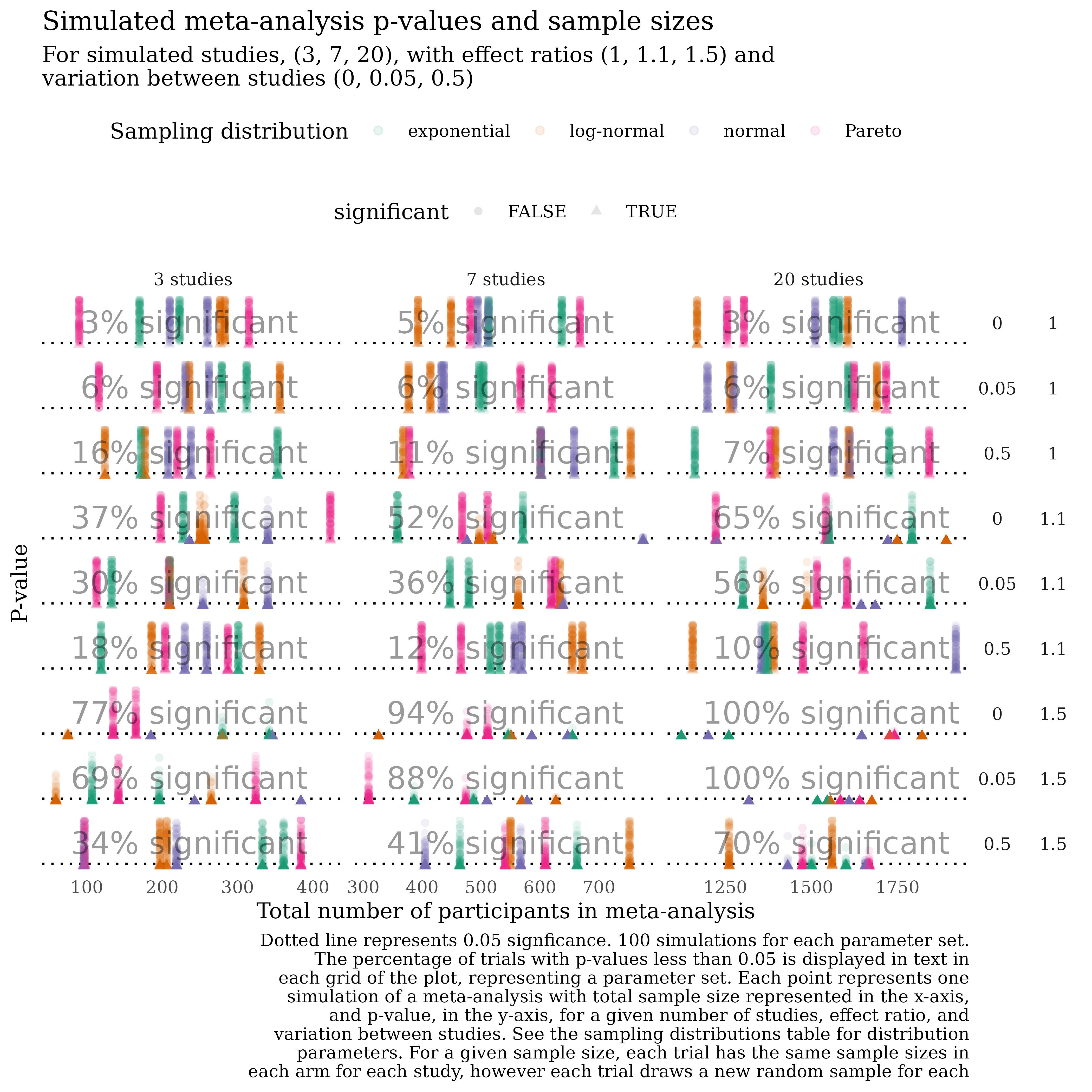
simulation walkthrough
include_graphics("man/figures/example_pipeline.png")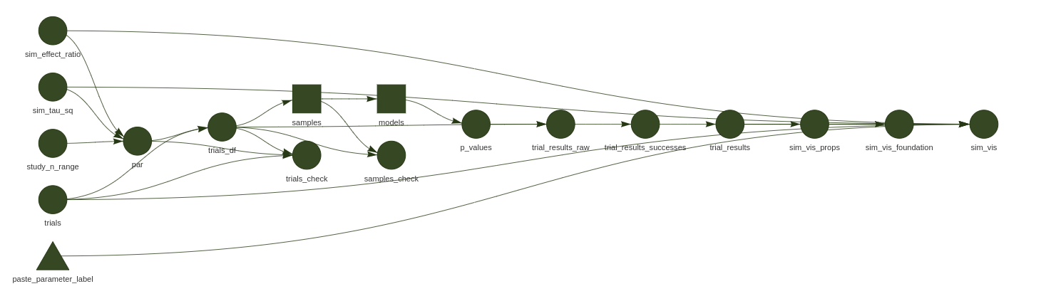
dim(trial_results)
#> [1] 21596 12
# move to
trial_results %>%
group_by(sim_id) %>%
summarise(
n_trials = n()
) %>%
full_join(trial_results, by = "sim_id", multiple = "all") %>%
select(-p_value_result, -dist_label) %>%
head()
#> # A tibble: 6 × 11
#> sim_id n_trials k tau_sq_true effect_…¹ rdist parameters parti…² study…³
#> <chr> <int> <dbl> <dbl> <dbl> <chr> <list> <int> <fct>
#> 1 sim 1 100 3 0 1 pare… <named list> 90 3 stud…
#> 2 sim 1 100 3 0 1 pare… <named list> 90 3 stud…
#> 3 sim 1 100 3 0 1 pare… <named list> 90 3 stud…
#> 4 sim 1 100 3 0 1 pare… <named list> 90 3 stud…
#> 5 sim 1 100 3 0 1 pare… <named list> 90 3 stud…
#> 6 sim 1 100 3 0 1 pare… <named list> 90 3 stud…
#> # … with 2 more variables: p_value <dbl>, significant <lgl>, and abbreviated
#> # variable names ¹effect_ratio, ²participants, ³study_n_labelSome details
Without specification, the function uses the default parameters dataset (?default_parameters).
| dist | par |
|---|---|
| pareto | 2, 1 |
| norm | 50, 17 |
| lnorm | 4.0, 0.3 |
| exp | 10 |
| pareto | 3.576119, 2.745808 |
| norm | 75.209383, 6.739041 |
| lnorm | 2.3900182, 0.3383603 |
| exp | 4.86717 |
This dataset also provides a template for how to set up a dataframe specifying the distributions and parameters of interest for sim_df. The default sampling distributions are designed to provide a mix of common symmetric and asymmetric families, with both fixed and randomly-generated parameters.
sim_dat <-
  # defaults to using default_parameters if we do not specify dist_df argument
  sim_df(
  # different effect sizes
  # what is small, medium large effect
  effect_ratio = sim_effect_ratio,
  # what is small medium large variance
  tau_sq = sim_tau_sq,
  min_n = sim_min_n,
  max_n = sim_max_n
)
# take a look at the top of the dataset
sim_dat %>% head(3)
#> # A tibble: 3 × 7
#>       k tau_sq_true effect_ratio rdist  parameters       n                sim_id
#>   <dbl>       <dbl>        <dbl> <chr>  <list>           <list>           <chr>
#> 1     3           0            1 pareto <named list [2]> <tibble [6 × 3]> sim 1
#> 2     3           0            1 norm   <named list [2]> <tibble [6 × 3]> sim 2
#> 3     3           0            1 lnorm  <named list [2]> <tibble [6 × 3]> sim 3

# the end of the dataset
sim_dat %>% tail(3)
#> # A tibble: 3 × 7
#>       k tau_sq_true effect_ratio rdist parameters       n                 sim_id
#>   <dbl>       <dbl>        <dbl> <chr> <list>           <list>            <chr>
#> 1    20         0.2          1.5 norm  <named list [2]> <tibble [40 × 3]> sim 94
#> 2    20         0.2          1.5 lnorm <named list [2]> <tibble [40 × 3]> sim 95
#> 3    20         0.2          1.5 exp   <named list [1]> <tibble [40 × 3]> sim 96

# take a look at a random handful of rows
sim_dat %>% sample_n(5)
#> # A tibble: 5 × 7
#>       k tau_sq_true effect_ratio rdist  parameters       n                sim_id
#>   <dbl>       <dbl>        <dbl> <chr>  <list>           <list>           <chr>
#> 1     3         0            1.5 pareto <named list [2]> <tibble [6 × 3]> sim 49
#> 2    20         0.2          1   norm   <named list [2]> <tibble>         sim 46
#> 3     7         0            1.5 exp    <named list [1]> <tibble>         sim 64
#> 4     3         0.2          1   lnorm  <named list [2]> <tibble [6 × 3]> sim 27
#> 5     3         0            1   lnorm  <named list [2]> <tibble [6 × 3]> sim 7
sim_df uses sim_n as explained below to create each dataset of sample sizes.
simulate paired sample sizes
This is a function I have often wished I’ve had on hand when simulating meta-analysis data. Thing is, running, say, 1000 simulations, I want to do this for the same sample sizes. So, I need to generate the sample sizes for each study and for each group (control or intervention).
Given a specific k, generate a set of sample sizes.
| study | group | n |
|---|---|---|
| Estelmo_1960 | control | 89 |
| Snaga_1953 | control | 20 |
| Théoden_1959 | control | 76 |
| Estelmo_1960 | intervention | 91 |
| Snaga_1953 | intervention | 20 |
| Théoden_1959 | intervention | 77 |
| study | group | n |
|---|---|---|
| Núneth_2002 | control | 68 |
| Folcred_1957 | control | 105 |
| Boromir_1957 | control | 14 |
| Núneth_2002 | intervention | 64 |
| Folcred_1957 | intervention | 93 |
| Boromir_1957 | intervention | 14 |
| study | group | n |
|---|---|---|
| Gwaihir_2002 | control | 42 |
| Amarië_1964 | control | 80 |
| Nori_1964 | control | 42 |
| Salmar_1987 | control | 92 |
| Anárion_1973 | control | 62 |
| Ulwarth_2007 | control | 95 |
| Gwaihir_2002 | intervention | 43 |
| Amarië_1964 | intervention | 67 |
| Nori_1964 | intervention | 33 |
| Salmar_1987 | intervention | 99 |
| Anárion_1973 | intervention | 59 |
| Ulwarth_2007 | intervention | 93 |
| study | group | n |
|---|---|---|
| Telchar_1972 | control | 14 |
| Asgon_1998 | control | 14 |
| Vëantur_1955 | control | 18 |
| Telchar_1972 | intervention | 16 |
| Asgon_1998 | intervention | 11 |
| Vëantur_1955 | intervention | 18 |
We expect cohorts from the same study to have roughly the same size, proportional to that size. We can control this proportion with the prop argument.
Suppose we wish to mimic data for which the cohorts are almost exactly the same (say becaues of classes of undergrads being split in half and accounting for dropouts).
| study | group | n |
|---|---|---|
| Beren_1979 | control | 28 |
| Azog_2013 | control | 19 |
| Beren_1979 | intervention | 2 |
| Azog_2013 | intervention | 1 |
It can be useful, for more human-interpretable purposes, to display the sample sizes in wide format.
simulation parameters
Adding a few values of τ, different numbers of studies k, and so forth can ramp up the number of combinations of simulation parameters very quickly.
I haven’t settled on a way of simulating data, and haven’t found heaps in the way of guidance yet. So, this is all a bit experimental. My guiding star is packaging what I’d use right now.
What I do always end up with is generating a dataset that summarises what I would like to iterate over in simulation.
The sim_df takes user inputs for distributions, numbers of studies, between-study error τ, within-study error ε, and the proportion ρ of sample size we expect the sample sizes to different within study cohorts.
# defaults
sim_df()
#> # A tibble: 216 × 7
#>        k tau_sq_true effect_ratio rdist  parameters       n        sim_id
#>    <dbl>       <dbl>        <dbl> <chr>  <list>           <list>   <chr>
#>  1     3           0            1 pareto <named list [2]> <tibble> sim 1
#>  2     3           0            1 norm   <named list [2]> <tibble> sim 2
#>  3     3           0            1 lnorm  <named list [2]> <tibble> sim 3
#>  4     3           0            1 exp    <named list [1]> <tibble> sim 4
#>  5     3           0            1 pareto <named list [2]> <tibble> sim 5
#>  6     3           0            1 norm   <named list [2]> <tibble> sim 6
#>  7     3           0            1 lnorm  <named list [2]> <tibble> sim 7
#>  8     3           0            1 exp    <named list [1]> <tibble> sim 8
#>  9     7           0            1 pareto <named list [2]> <tibble> sim 9
#> 10     7           0            1 norm   <named list [2]> <tibble> sim 10
#> # … with 206 more rows

sim_df() %>% str(1)
#> tibble [216 × 7] (S3: tbl_df/tbl/data.frame)

# only consider small values of k
sim_df(k = c(2, 5, 7)) %>% str(1)
#> tibble [216 × 7] (S3: tbl_df/tbl/data.frame)
For the list-column of tibbles n, the sim_df function calls sim_n and generates a set of sample sizes based on the value in the column k.
demo_k <- sim_df()

# the variable n is a list-column of tibbles
demo_k %>% pluck("n") %>% head(3)
#> [[1]]
#> # A tibble: 6 × 3
#>   study        group            n
#>   <chr>        <chr>        <dbl>
#> 1 Mandos_2000  control         23
#> 2 Niënor_1955  control         62
#> 3 Yavanna_2015 control         17
#> 4 Mandos_2000  intervention    25
#> 5 Niënor_1955  intervention    70
#> 6 Yavanna_2015 intervention    19
#>
#> [[2]]
#> # A tibble: 6 × 3
#>   study       group            n
#>   <chr>       <chr>        <dbl>
#> 1 Aravir_1953 control         35
#> 2 Anborn_1982 control         74
#> 3 Elphir_1984 control         17
#> 4 Aravir_1953 intervention    34
#> 5 Anborn_1982 intervention    71
#> 6 Elphir_1984 intervention    17
#>
#> [[3]]
#> # A tibble: 6 × 3
#>   study        group            n
#>   <chr>        <chr>        <dbl>
#> 1 Aragost_1981 control         67
#> 2 Orcobal_1994 control         88
#> 3 Khîm_1954    control         15
#> 4 Aragost_1981 intervention    64
#> 5 Orcobal_1994 intervention    82
#> 6 Khîm_1954    intervention    16


# compare the number of rows in the dataframe in the n column with the k value
# divide by two because there are two rows for each study,
# one for each group, control and intervention
demo_k %>% pluck("n") %>% map_int(nrow) %>% head(3) / 2
#> [1] 3 3 3
demo_k %>% pluck("k") %>% head(3)
#> [1] 3 3 3
simulating data
Once we have established a set of sample sizes for a given distribution, with parameters, and so forth, I usually want to generate a sample for each of those n. We need to adjust the value of the sampled data based on the median ratio, and whether the n is from a control or intervention group.
A random effect is added to account for the between study error τ and within study error ε.
For meta-analysis data, we work with summmary statistics, so we drop the sample and return tabulated summary stats.
| study | effect_c | effect_spread_c | n_c | effect_i | effect_spread_i | n_i |
|---|---|---|---|---|---|---|
| Bob_2004 | 58.77079 | 0.2146638 | 48 | 51.03713 | 0.1810027 | 42 |
| Oromë_1981 | 49.68544 | 0.2232972 | 45 | 60.28628 | 0.1896956 | 43 |
| Ufthak_1965 | 68.67402 | 0.2019829 | 42 | 43.72458 | 0.1893396 | 48 |
Archived PhD work (see phd-scripts/)
trial
In a trial, we’d first want to simulate some data, for a given distribution, for this we use the sim_stats function discussed in the above section.
With the summary statistics, we then calculate an estimate of the effect or the variance of the effect.
- simulate data
- calculate summary statistics
- calculate estimates using summary statistics
- calculate effects using estimates (difference, standardised, log-ratio)1
- meta-analyse
- return simulation results of interest
The first two steps are taken care of by the sim_stats function. The third step will by necessity be bespoke.
But the rest could be automated, assuming there are the same kinds of results.
| step | input | output |
|---|---|---|
| calculate estimates | summary statistics as produced by sim_n
|
summary stats |
| calculate effects | summary stats |
effect and effect_se
|
| meta-analyse |
effect and effect_se
|
rma object |
| summary stats |
rma object |
some kind of brooming script |
metatrial()summarising simulation results
So, now we can put together some generic summarisations. Things I always want to do. Like calculate the coverage probability, confidence interval width, and bias. Most results here are mean values across all trials, the exceptions being cp_ variables.
metasim calls metatrial many times and summarises the results.
metasim()visualise
sim %>% coverage_plot()Ideally this would be configurable but let’s hardcode it for now.↩︎