A singularity of button

Author

Affiliation

Dr Charles T. Gray, Datapunk

Good Enough Data & Systems Lab

Published

March 14, 2025

The button problem

So, where to start with the button problem?

Code

# pkg
library(tidyverse)
library(ggraph)
library(tidygraph)

I get agile.

But, as a human, I feel overwhelmed.

Think of agile like this. 

Leadership: Mirror, mirror on  the  wall, 
  who has the FAIRest vision of them all?

Product managers smash the mirror into pieces.

Developers smash those pieces into shards.

Different developers paint the shards in 
  tiny ways to make the vision FAIR.

Developers reassemble shards into pieces.

Product managers reassemble those pieces 
  into the mirror painted to leadership's vision.

Leadership: Mirror, mirror on the wall, forget FAIR, 
  I can't see my fucking face at all.

I can see why there was a breakdown between humans. I can see how flat/vertical cultural differences come into play.

But why is there an analogous breakdown for me developing alone?

Why do I feel like the greater my computational projects scale, the greater the anxiety? Why does nothing ever go as it should?

It’s the not knowing that drives me crazy. If I could just know what I know, at least see what the bounds of knowledge of this system is, I think I would feel less overwhelmed.

The answer is in chaos and category theory. Let’s go. Freeform.

Singularities within the button problem

button visualisatons
formatting across slides and manuscript did not work
game
slides
manuscript

Button characteristics

These are all supported by the button package.

Fundamentally, there’s something to be learnt from the music project.

What went wrong?

Assumption as a graph, $B$ .

It always starts with edges.

output key assumption: dataframe has fromand to.

Code

B_edges <-
  tribble(
    ~from,    ~to,
    "raw",    "edges",
    "edges",  "nodes",
    "raw",    "nodes",
    "edges",  "tidygraph",
    "nodes",  "tidygraph",
    "tidygraph", "ggraph",
    "ggraph",   "display",
    "display",  "deploy"
  )

Code

# check assumption
colwise_check <- c("from", "to") %in% colnames(B_edges) 

colwise_check

[1] TRUE TRUE

Code

# convert colwise vector to boolean
all(colwise_check) == TRUE

[1] TRUE

Code

# display edges
B_edges

# A tibble: 8 × 2
  from      to       
  <chr>     <chr>    
1 raw       edges    
2 edges     nodes    
3 raw       nodes    
4 edges     tidygraph
5 nodes     tidygraph
6 tidygraph ggraph   
7 ggraph    display  
8 display   deploy

Then node metadata often needs to be extracted or inferred.

A challenge is node joining happens after the graph object is created.

output key assumption: there is exactly one row per node in B_edges

Code

B_nodes <-
  # extract nodes from edges
  tibble(
    node = c(B_edges$from, B_edges$to)
  ) |>
  # filter to unique nodes
  distinct() |>
  # add node attributes
  mutate(
    # necessary
    node_label = node,

    # contextual
    painpoint = if_else(
      node %in% c("deploy", "tidygraph"),
      TRUE,
      FALSE
    ),
    node_emergence = if_else(
      painpoint == TRUE,
      "miscreant",
      "expected"
    )
  )

the antijoin nodes and edges by node should have no rows

Code

B_antijoin <-
  {
    tibble(
      node = c(B_edges$from, B_edges$to)
    ) |>
    # filter to unique nodes
    distinct()
  } |> anti_join(B_nodes |> select(node), by = "node")

verify assumption

Code

nrow(B_antijoin) == 0

[1] TRUE

display nodes

Code

B_nodes

# A tibble: 7 × 4
  node      node_label painpoint node_emergence
  <chr>     <chr>      <lgl>     <chr>         
1 raw       raw        FALSE     expected      
2 edges     edges      FALSE     expected      
3 nodes     nodes      FALSE     expected      
4 tidygraph tidygraph  TRUE      miscreant     
5 ggraph    ggraph     FALSE     expected      
6 display   display    FALSE     expected      
7 deploy    deploy     TRUE      miscreant

Code

B_graph <- 
  B_edges |>
  as_tbl_graph() |>
  activate(nodes) |>
  # add node attributes
  left_join(B_nodes, by = c("name" = "node"))

B_graph

# A tbl_graph: 7 nodes and 8 edges
#
# A directed acyclic simple graph with 1 component
#
# Node Data: 7 × 4 (active)
  name      node_label painpoint node_emergence
  <chr>     <chr>      <lgl>     <chr>         
1 raw       raw        FALSE     expected      
2 edges     edges      FALSE     expected      
3 nodes     nodes      FALSE     expected      
4 tidygraph tidygraph  TRUE      miscreant     
5 ggraph    ggraph     FALSE     expected      
6 display   display    FALSE     expected      
7 deploy    deploy     TRUE      miscreant     
#
# Edge Data: 8 × 2
   from    to
  <int> <int>
1     1     2
2     2     3
3     1     3
# ℹ 5 more rows

Code

B_graph |>
  ggraph() +
  geom_edge_link(
    arrow = arrow(
      length  = unit(0.02, "npc"),
      angle = 20
      ),
    alpha = 0.3,
    start_cap = circle(0.03, 'npc'),
    end_cap = circle(0.03, 'npc')
  ) +
  geom_node_point(
    aes(colour = node_emergence)
  ) +
  geom_node_text(
    aes(label = node_label),
    repel = TRUE,
    family = "Courier"
  ) +
  theme_minimal() +
  theme(
    plot.title = element_text(
      family = "Courier"
      ),
    plot.subtitle = element_text(
      family = "Courier"
      ),    
    plot.caption = element_text(
      family = "Courier"
      ),    
    axis.text = element_blank(),
    axis.title = element_blank(),
    panel.grid = element_blank()
  ) +
  labs(
    title = "Development Expectation",
    subtitle = "Known problems at tidygraph and deployment"
  ) +
  ggplot2:::manual_scale(
    "colour",
    values = setNames(
      c("#a6611a", "#018571","#dfc27d", "#80cdc1"),
      c("violation", "virtuous", "miscreant", "expected")
    )
  )

Using "sugiyama" as default layout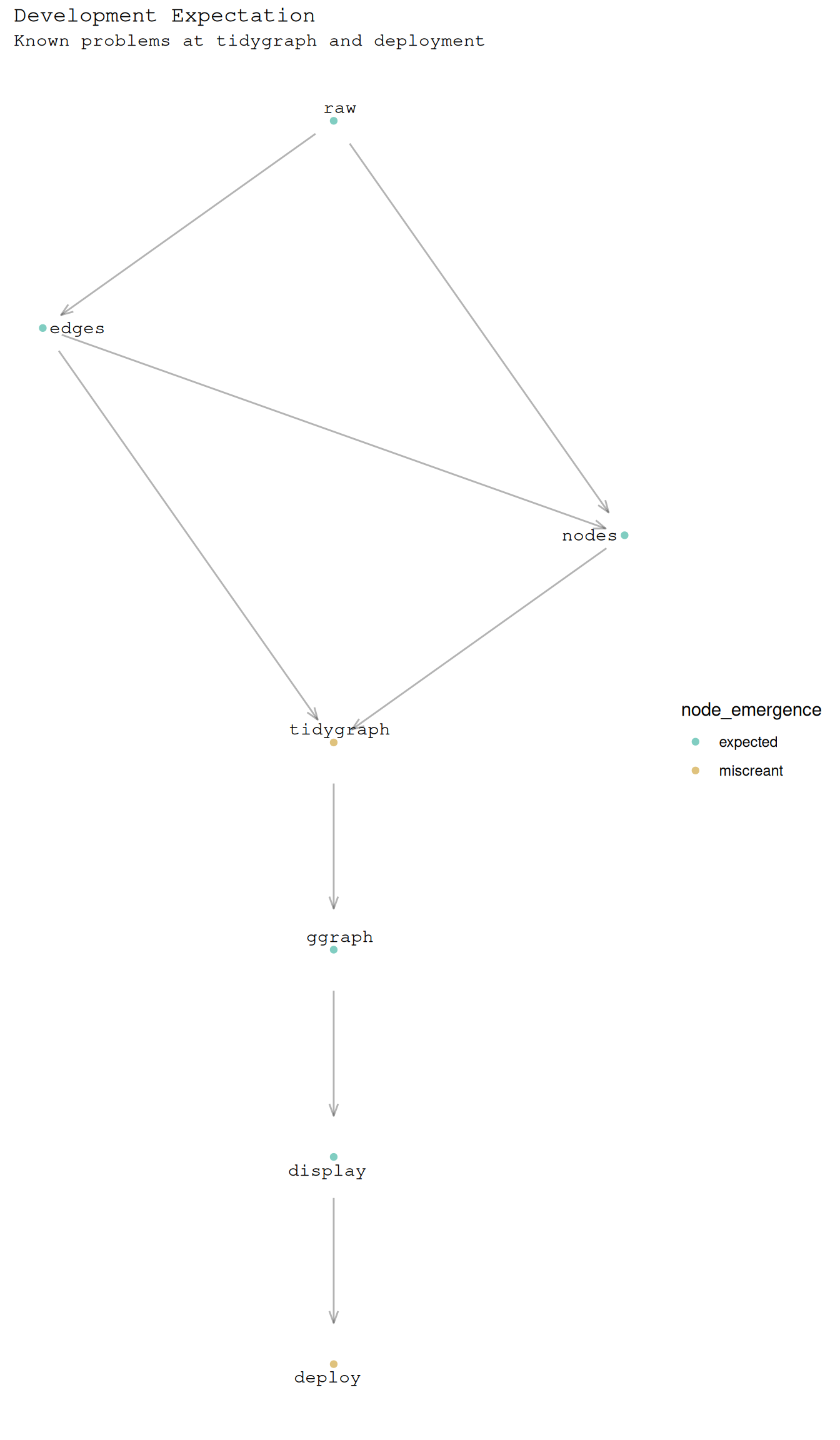

Experimented with api-ing some data in. Promising.